Real-Time Chatter Detection

The problem

Chatter happens when a cutting tool and the machine structure fall into a self-excited feedback loop. Vibration amplitude grows fast, surface finish is ruined, and tools and spindles wear out. The physics is well understood through regenerative chatter theory and stability-lobe diagrams. Detecting it live, from a noisy sensor, fast enough to react, is still hard.

The task I set:

Train on clean simulated cuts.
Detect chatter on cuts corrupted with realistic sensor noise the model never saw.
Use only the signal. Spindle speed, depth of cut and natural frequency define the ground-truth label, so feeding any of them to the model would leak the answer.
Decide every 50 ms, with inference well inside a 100 ms control budget.

I work with Prof. Tony Schmitz and Dr. Michael Gomez of MSC Industrial and the University of Tennessee Machine Tool Research Center, who generated simulation datasets to stress-test the model.

Approach

Physics-informed features

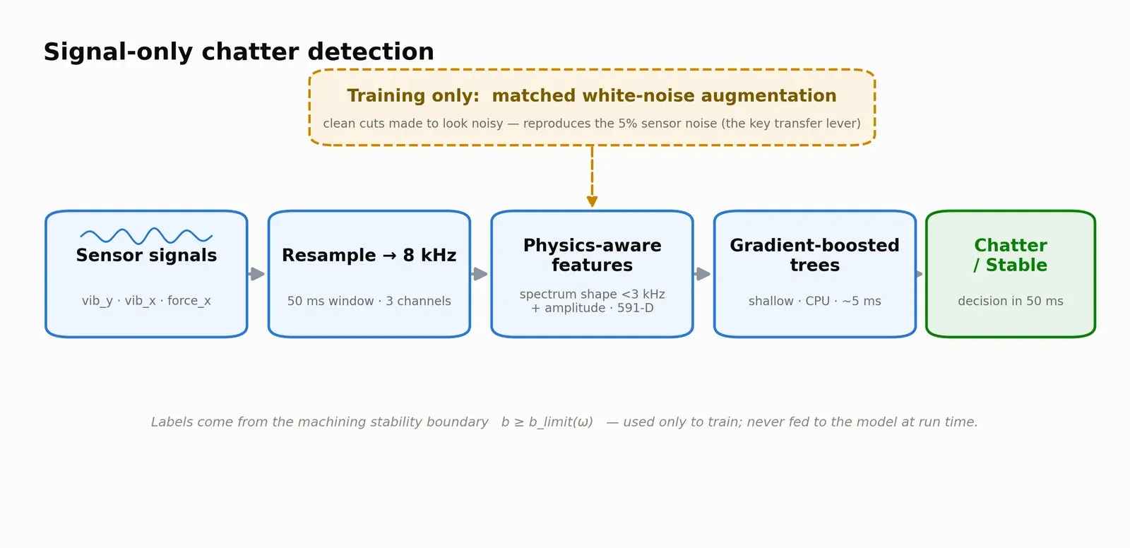
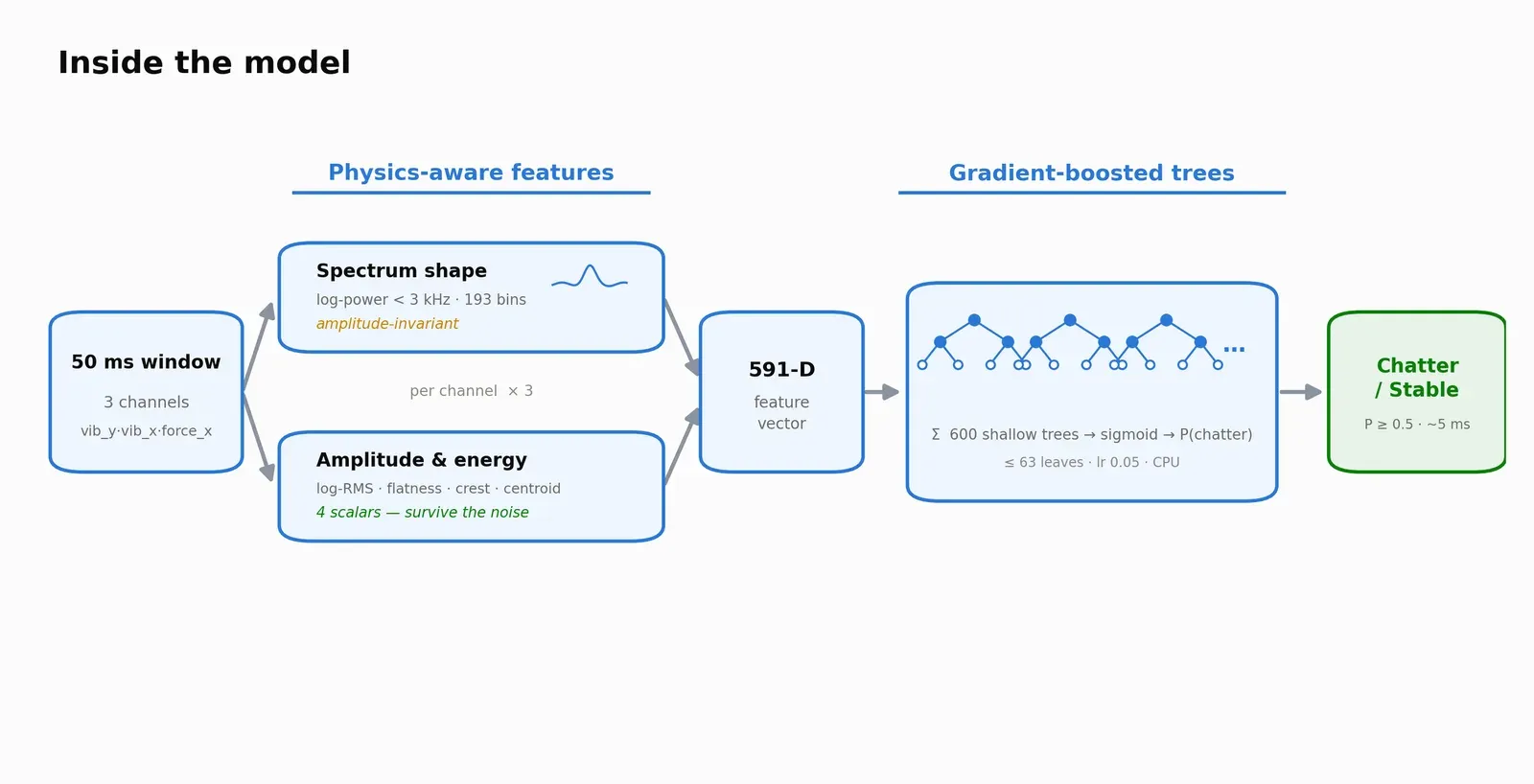
Each 50 ms window has three channels: two vibration axes and cutting force. I turn each window into features a machining engineer would recognize:

An amplitude-invariant log-power spectrum. When the cut is stable, energy sits on the tooth-passing orders. When it chatters, energy piles up at a chatter frequency near a structural mode.
A few amplitude and energy descriptors: RMS, spectral flatness, crest factor and spectral centroid.

The signal-only detection pipeline — The signal-only pipeline: three channels per 50 ms window, physics-informed features, the model, and a stable or chatter decision.

What I tried first

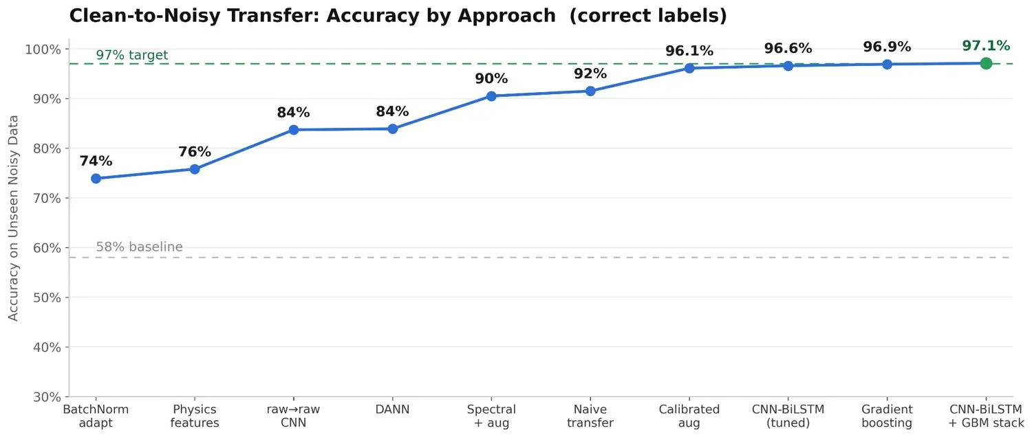
Before settling on features plus augmentation, I tried the standard domain-adaptation routes. Adapting batch-norm statistics to the noisy domain reached 74%. A CNN on raw signals and a domain-adversarial network (DANN) both stalled at 84%. Calibrated noise augmentation reached 96.1%, so I built on that.

Matched-noise augmentation

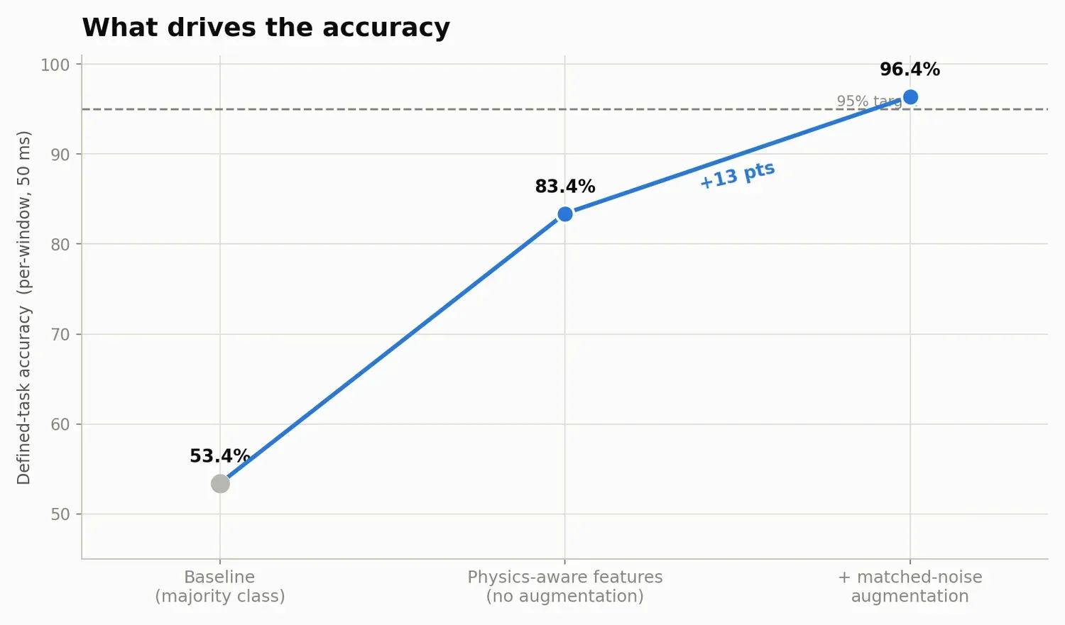
I measured the sensor noise and found it white, proportional to the signal, and RMS-preserving. That means absolute amplitude survives the noise and is a cue the model can transfer. Training with synthetic noise matched to that measured statistic was the biggest single lever in the project. It closed most of the clean-to-noisy gap and added 13 points of accuracy.

A stacked ensemble

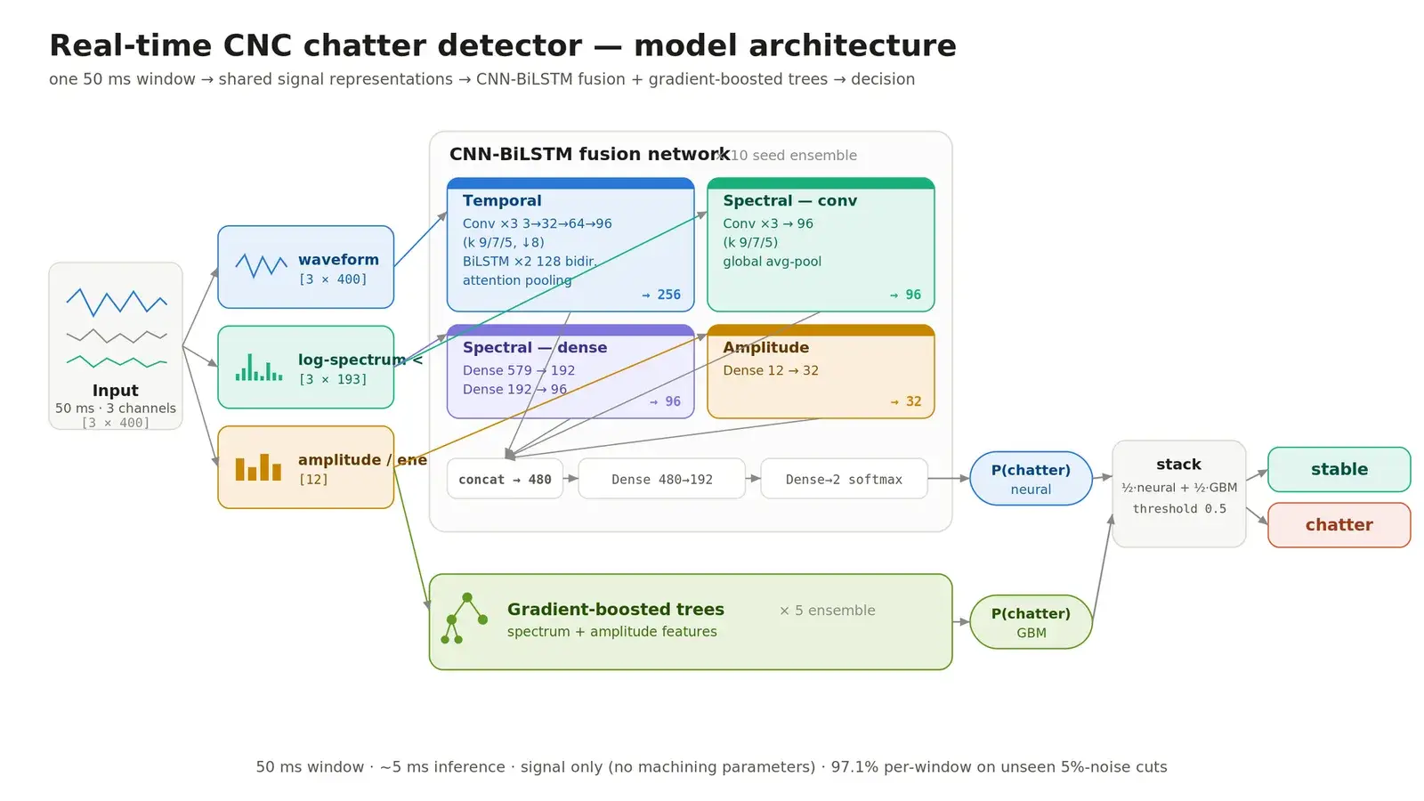
Two learners read the same window and I average their probabilities:

a CNN-BiLSTM fusion network with temporal, spectral and amplitude branches;
a gradient-boosted-tree ensemble on the physics features.

They make different mistakes, so the stack beats either one alone. The tree half is auditable: you can see which physical features drive each decision. The whole stack runs on one window in about 5 ms on a commodity CPU.

Physics-aware features feeding the tree ensemble — The physics-aware features and the gradient-boosted-tree branch, which runs in parallel with the deep network.

Results

Trained on clean cuts and tested on unseen cuts with 5% noise, with no retraining:

Setting	Accuracy
Defined task, clean to noisy, per window	97.1% stacked, 96.9% trees only
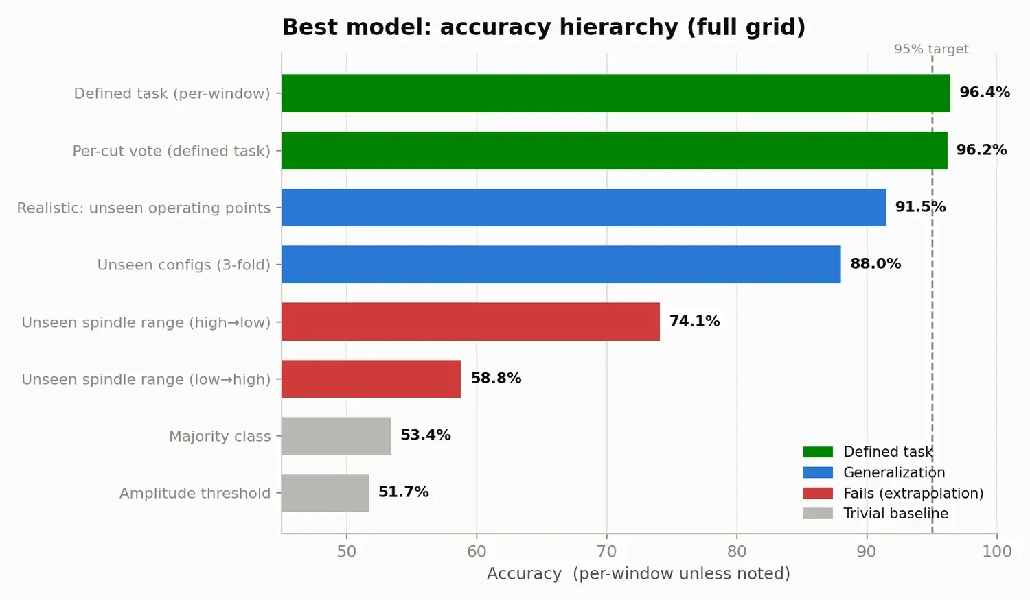
Unseen operating points, same machine	91.5%
Unseen configurations with new natural frequencies	88 to 90%
Trivial baselines (majority class, amplitude threshold)	52 to 58%
Inference time	~5 ms per 50 ms window

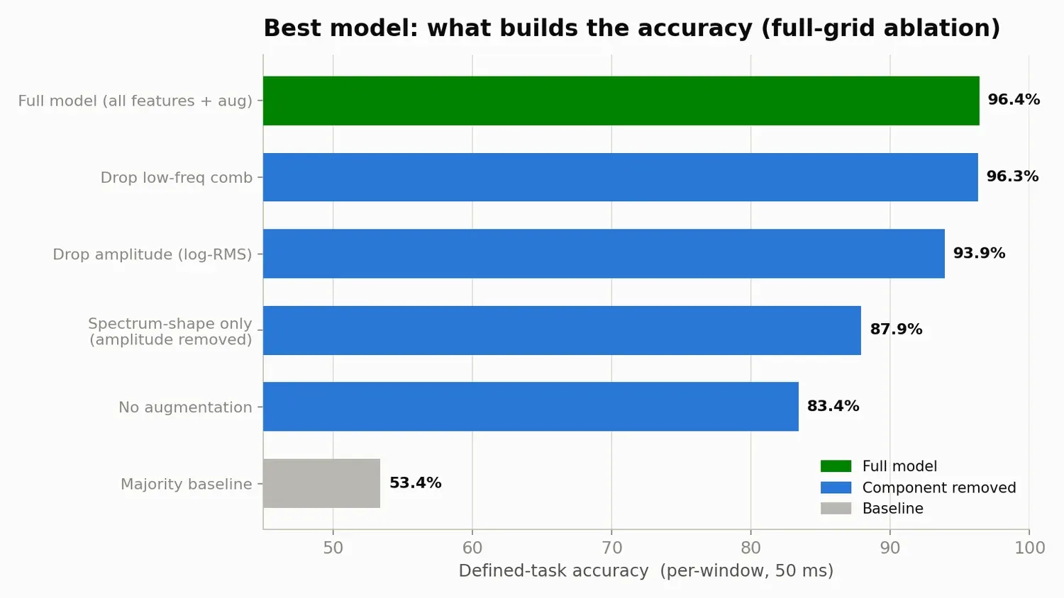
Clean-to-noisy transfer from 58% to 97.1% — Every approach I tried for clean-to-noisy transfer, scored on unseen noisy data. Domain adaptation stalled at 74 to 84%. Calibrated augmentation reached 96.1%, and the CNN-BiLSTM plus gradient-boosting stack reached 97.1%, against a 58% baseline.

Accuracy hierarchy of the best single model — The best single model across the full grid: 96.4% on the defined task, 91.5% on unseen operating points and 88.0% on unseen configurations. It fails when extrapolating to spindle-speed ranges it never trained on (74.1% and 58.8%).

A removal ablation shows each component earns its place. With amplitude removed, spectrum shape alone still reaches 87.9%, so the model is detecting the chatter frequency in the spectrum as well as reacting to amplitude.

Ablation of the model components — Removal ablation on the best single model: dropping amplitude costs 2.5 points, spectrum shape alone reaches 87.9%, and training without augmentation falls to 83.4%.

Where it fails

It does not extrapolate to spindle-speed ranges it never trained on (74.1% high-to-low, 58.8% low-to-high in the figure above).
Accuracy dips right at the stability boundary. That region is physically ambiguous because chatter grows continuously from zero. Clear-cut cases score 98 to 99%.

Checking my own numbers

I re-derived every window’s label from the stability physics and found zero mismatches across about 51,000 windows per domain. Matched clean and noisy pairs agree exactly.
When a new dataset scored 100%, I traced it: about 90% of its operating points were effectively training points at a new noise level, with a 0.9997 correlation to the training signals. I corrected the reported number.

Extending to unseen spindle speeds

Using methods from my collaborators (self-differencing to remove periodic content, and the Honeycutt-Schmitz periodic-sampling stability metric), I built a frequency-scaling augmentation around the fact that chatter is not synchronous with tool rotation. It improved the hardest zero-shot case, unseen spindle speeds, by 10 points with almost no loss inside the training envelope.

Deployment and testing

The detector runs as a ROS 2 node in rclpy. It buffers a live sensor stream, keeps a sliding 50 ms window with a 25 ms step, resamples to a common rate, extracts the features, runs the model, and publishes a chatter probability and a boolean flag. The tree path is CPU-only and feed-forward, so streaming needs no recurrence. On replayed real cuts it agreed with ground truth 100% of the time.

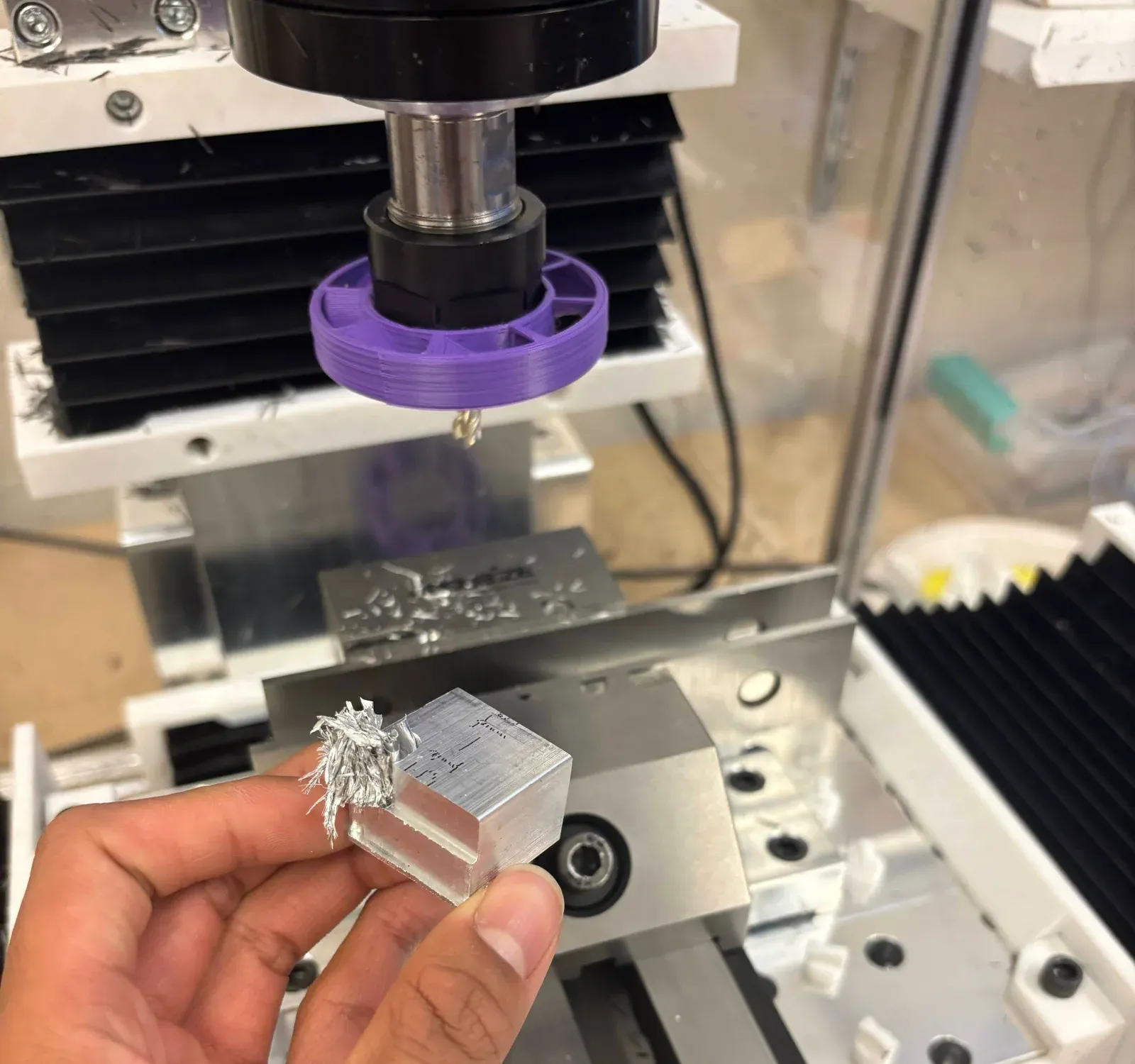
The detector is validated mainly on high-fidelity physics simulation. Real-world testing has started: early tests used a microphone, and we have collected accelerometer data from cuts. The next step is testing on Autodesk’s machines with their accelerometer vibration data.

An aluminum test block held beside a benchtop mill after a cut — An aluminum test block after a cut on a benchtop mill, from the early real-world testing.

Recognition

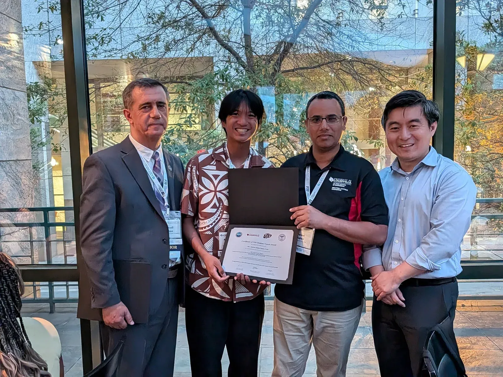
The work earned a National Science Foundation travel grant, presented by the Society of Manufacturing Engineers (SME). We interviewed a machinist at Apple about the problem, and Autodesk and GE Vernova have offered their machines for testing.

AJ receiving the NSF travel grant certificate with three presenters — Receiving the NSF travel grant, presented by SME, for this work.

My contribution

I built the detector alone: the dataset handling and label checks, the feature pipeline, both models and the stack, the augmentation studies, the ablations and the ROS 2 node. My collaborators at MSC Industrial and the University of Tennessee generated the simulation datasets and contributed the signal-processing methods I adapted for the spindle-speed augmentation.